The color map is a property of the matrix plot and all aspects of the color map is
accessed through the "MatrixPlot::colormap" property which is an
instance of class MatrixColormap.
To adjust how the color map is used the following methods are available
-
ColorMap::SetMap($aMap, $aInvert=false)This is a polymorphic method that can take either a symbolic constant as argument and in that case specifies one of the built in color maps or it can be an array of colors which in that case specifies a manual color map. There are several built in color maps of different types which are referenced by an integer in range [0, 19]. A list of the built in color maps can be found in Built in color maps
For example the specification
1
$mp->colormap->SetMap(0);will make the library use the heat color map which is standard color map that goes from black for the min value up through red, orange, yellow and finally white for the highest value. This could be though of as the color of a heated iron rod (the hottest iron is white glowing).
The following manual specification uses three color plateau that the map touches.
1
2
$map = array( 'navy', 'gray', 'red' );
$mp->colormap->Set($map);
would create a color map that would use '
navy' color for the min value and 'red' for the max value and linearly interpolate all other values for a color range continuously moving from 'navy'-'gray'-'red'. The color interpolation made between these values is a linear interpolation of the corresponding RGB values which creates the illusion of a continuous color change. The array must have at least two colors. There is no limit on the maximum number of base colors specified. However using more than ~7-10 colors to specify the color map is probably not to be recommended.If
$aInvertis set totruethen the color map will be reversed so that the lowest color in the map will be the highest and vice versa. -
ColorMap::GetCurrMap()Return the current set color map
-
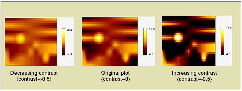
ClorMap::SetRange($aMin,$aMax)This is used to manually specify the min and max values to be used for mapping matrix values to a color. Any values in the matrix that is lower than
$aMinwill be set to the min color and any values above$aMaxwill be set to the maximum color.The matrix values in between will be mapped to the entire color scale. Another way of looking at this is that this will compress the dynamic range used or the colors. If the min and max values specified are much higher and lower than the actual content of the matrix the result is that most of the colors in the matrix will have "middle" colors (and hence lower the contrast). By default the values are (0,0) which means that the library will automatically determine the min/max value based on the input data and use the entire range of colors specified in the color map.
1
2
3
4
5
6
7
8
// This will lower the contrast by roughly 50 percent $mindataval = ... ; // The minimum data value $maxdataval = ... ; // The maximum data value $contrast = -0.5; // Reduce the contrast by 50% $adj = ($maxdataval-$mindataval+1)*$contrast/2; $matrixplot->colormap->SetRange($mindataval+$adj, $maxdataval-$adj);
In a similar way the following code will instead increase the "contrast" 50% by letting a large part of the data values become mapped to the min and max color values.
1
2
3
4
5
6
7
8
// This will increase the contrast by roughly 50 percent $mindataval = ... ; // The minimum data value $maxdataval = ... ; // The maximum data value $contrast = 0.5; // Increase the contrast by 50% $adj = ($maxdataval-$mindataval+1)*$contrast/2; $matrixplot->colormap->SetRange($mindataval+$adj, $maxdataval-$adj);
The three plots in Figure 22.3. The effects of changing the value range for the colormap shows the effect of increasing and decreasing the contrast with this method.
Tip
When using the auto ranging (the default) the contrast can be adjusted with a call to
-
MatrixPlot::SetAutoContrast($aContrast)
as in
1
$matrixplot->SetAutoContrast(-0.3); -
-
ColorMap::SetNumColors($aNum)This is used to specify the number of discrete color steps used in the map. By default the scale range is divided in approximately 64 color buckets that all matrix entries are mapped into. Depending on the actual color map the specified value might be adjusted up or down up to +/- (p-1). Where p=number of base colors. Valid ranges are 3-128 but is also dependent on the actual color map.
The reasons for these restriction and the adjustments are
-
The minimum number of colors are the number of base colors in the current color map
-
The number of colors must satisfy the equation
n = p + k*(p-1), k = 0, 1, 2, ... (eq. 1)
where
-
n = number of colors
-
p = number of base colors that specifies the map
The specified number of colors will be adjusted to the closest number that satisfies (eq. 1).
-
-
-
ColorMap::SetNullColor($aColor)If specified this determines what color will be used for any values in the matrix that are null
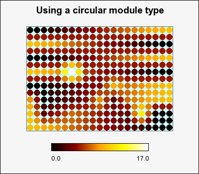
By default the module type (the shape that represents one cell in the matrix) is a rectangle. As was mentioned in the introduction this can also be a circle. This is controlled by the method
-
MatrixPlot::SetModuleType($aType)$aType, 0 = Use rectangle, 1 = Use a circle
When using circular module type it might also be useful to specify a separate background color for the plot since there will be some space between the circles where the background can be seen. The plot background is specified with the method
-
MatrixPlot::SetBackgroundColor($aColor)
An example of using circular modules can be seen in Figure 22.4. Using a circular module type ( matrix_ex05.php)
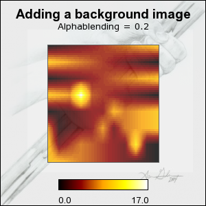
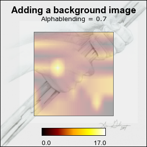
By default the plots are filled with solid colors from the chosen color map. By specifying an alpha value it is possible to let the background shine through the matrix plot. The alpha blending is chosen by the method
-
MatrixPlot::SetAlpha($aAlpha)$aAlpha, 0=No transparency, 1=Full transparency (not so useful since then only the background can be seen)
|
|
|
Note
As can be seen in the figures only the plot area is adjusted. The legend is always shown with no transparency.
There are three and disjunct way to specify the size of the matrix plot. However the size can not be set to any pixel value. Since the matrix plot is a visualization of a matrix the width and height must always be an even multiple of the number of rows and columns since each cell in the matrix have an integer number of pixels as width and height (the module size). This will sometimes force the library to adjust a specified size so that it is an even multiple of the number of rows and columns in the input data matrix.
For example; if the matrix has 50 columns this means that the width will only grow and shrink by multiples of 50 pixels since each cell has an equal number of pixels. The minimum width for such a matrix is 50 pixels.
There are three ways to specify the size:
-
by setting the width and height explicitly (in number of pixels).
Note that the actual rendered size might be different depending on the input matrix size since each cell must have an integer number of pixels and not all sizes will be even dividable with the input data matrix size.
-
by setting the width and height as fractions of the overall width and height of the graph
Note that the actual rendered size might be different depending on the size of the input data matrix.
-
by specifying the width and height of each rendered cell (a.k.a the module size)
This specifies the size (in pixels) of each module. The minimum size is 1x1 pixels.
The size is adjusted by the following two methods
-
MatrixPlot::SetSize($aW,$aH)MatrixPlot::SetSize($aW)If the two arguments are numbers in range [0.0, 1.0] it will be interpreted as specifying the size as fractions of the overall graph width and height. If the number are > 1 they will be interpreted as the absolute size (in pixels). It is perfectly possible to mix teh two ways. For example the following is a valid size specification
1
$matrixplot->SetSize(250,0.6); // 250px wide and height will be ~60% of the graph heightIf only one argument is specified it will set both the width and height to the specified size. If the single size is specified as a fraction the smallest of the graph width/height will be used as the base.
-
MatrixPlot::SetModuleSize($aW,$aH)The two argument specifies the module size, i.e. the size of each cell in the plot (in pixels).
Note
The size does not effect the legend that belongs to a matrix plot.
The position of the plot by is by default centered vertically and slightly move to the left of the vertical center in order to compensate for the default legend that is shown n the right of the plot. The position of the plot is specified by the method
-
MatrixPlot::SetCenterPos($aX,$aY)Specifies the center of the plot to be the given x and y-coordinates. The position can be specified in either absolute pixels or as fractions of the width and height (or as a combination).
Tip
In order to position multiple plots on the same graph it is easier to user the layout classes (as described in Using layout classes to position matrix plots)
The legend belongs to the matrix plot and not the graph. All legend are instances
of class MatrixLegend and is accessed through the property
-
MatrixPlot::legend
By default the legend is enabled and positioned to the right of the plot. Both the size and position of the legend can be manually adjusted.
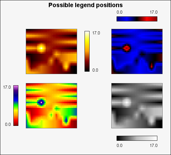
There are four possible positions of the legend as shown in Figure 22.7. Matrix legend positions, on each of the four sides of the plot. The labels of the legend will be automatically adjusted to face aways from the plot.
To position the legend the following MatrixPlot method is used
-
MatrixPlot::SetLegendLayout($aPos)The position of the legend is specified as an integer in range [0-3] where 0 is the right side of the plot and the remaining posiotins follow clockwise from the right, (i.e. 1 is the bottom, 2 is the left and 3 is the top side).
The following methods can be used to fine tune and adjust the legend
-
MatrixLegend::Show($aFlg=true)Used to enable/disable the legend. The following code line would hide the legend
1
$matrixplot->legend->Show(false); -
MatrixLegend::SetModuleSize($aBucketWidth,$aBucketHeight=5)This specifies the size of each color bucket in the legend.
-
MatrixLegend::SetSize($aWidth,$aHeight=5)This is an alternative way to specify the size of the legend compare with the individual bucket specification. With this method the overall width and height of the legend bar can be adjusted. The size can be specified s either absolute pixels or as fraction of the width height of the entire graph.
-
MatrixLegend::SetMargin($aMargin)Specifies the margin (in pixels) between the matrix plot and the legend.
-
MatrixLegend::SetLabelMargin($aMargin)Specifies the margin between the min/max label and the legend bar
-
MatrixLegend::SetFont($aFamily,$aStyle,$aSize)Specifies the font for the label on the legend
-
MatrixLegend::SetFormatString($aStr)Specifies the format string (in
printf()format) to be used when rendering the legend label
Note
This feature is only available in v3.0.4p and above.
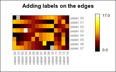
When using matrix plots to display micro arrays it is often desirable to have
legends for each row and column. Figure 22.8. Adding row and column legends to a matrix plot ( shows an example of this which helps
understand this concept.matrix_edgeex01.php)
In the library this is modelled by the class EdgeLabel which is
instantiated in the matrix plot as
-
MatrixPlot::collabelInstance for horizontal labels
-
MatrixPlot::rowlabelInstance for vertical labels
To adjust the appearance of the labels the following methods can be used:
-
EdgeLabel::SetFont($aFF,$aFS,$aSize)Specify the font to be used. Keep in mind that the font size should not be larger than the module size chosen to be able to fit within the row/column it specifies. For the default module size a font size of 8-9 for a TTF font is usually fine. By default the labels are set in FF_ARIAL, 8 pt size.
-
EdgeLabel::SetFontColor($aColor)Specifies the font color.
-
EdgeLabel::SetMargin($aMargin)Set the margin from the edge of the matrix in pixels.
-
EdgeLabel::SetSide($aSide)Specifies on what side the labels should be drawn. For horizontal (x) labels the possible sides are
"left"or"right"and for vertical (y) the possible sides are"top"and"bottom". -
EdgeLabel::Set($aLabels)Specifies the 1-dimensional array that holds the labels to be used.
-
EdgeLabel::SetAngle($aAngle)Specify the angle to draw the label at. By default row labels are drawn at 0 degree and column labels are drawn at 90 degrees angle.
The simplest use of labels is to use the default values for all parameters and just set the labels, i.e.
1 2 3 4 5 6 7 8 9 10 | $data = array( ... ) ; $collabels = array( ... ) ; $rowlabels = array( ... ) ; $mp = new MatrixPlot($data); $mp->collabel->Set($collabels); $mp->rowlabel->Set($rowlabels); |
Below is a final example of adding row and column labels to a matrix graph
1 | #=matrix_edgeex02|Adding row and column legends to a matrix plot## |